This is a project I completed with my friends [Akil Daresalamwala] and [Rudra Raval] for the 2024 NFL Big Data Bowl.
The Tackle Tango: An Analysis of Poise and Performance in Tackling
Introduction
Two of the largest pillars of football are carrying the ball and tackling the carrier. By this philosophy, tackling makes up half of the importance in the game we all love. With the plethora of factors that make up a tackle - from reading the play to shedding a block to velocity to a small loss of traction with the turf - it’s almost impossible to find a good correlation between a player’s characteristics and his ability to tackle well. However, by using historical tracking data and the real outcomes associated with it, we’re able to model good tackling while, to an extent, abstracting the nitty gritty details behind the mask of real-life data.
Theory
Tackling is a multi-stage process, which calls for a multi-stage analysis. To comprehensively analyze a tackle, we need to take into account how well defenders set themselves up to make the tackle, as well as how well they can bring the ball carrier down. We propose two metrics: Strategic Pursuit Evaluation for Effective Defense (SPEED) and Weighted Average Tackle Total (WATT), and combine them to make the Velocity Optimization and Rapid Tackle Execution (VORTEX) plot.
Data Cleaning
Before we get started, we need to clean up the dataset. This analysis serves as a proof of concept, and we chose to focus in on run plays. Also, since the name of the game is tackling, we consider only plays during which a tackle is made. Of these plays, the relevant portions are from the moment of handoff to the moment of tackle since otherwise, cornerbacks and safeties would be unfairly penalized for moving away from the ball to cover their man or zone. We filtered the data by these requirements to reduce runtime and make sure to fairly score players.
Approach
- Determine players who are eligible to be potential tacklers for any given play. It is incorrect to penalize players lined up across the field from a tackle for not being involved in said tackle.
- For the players who are potential tacklers, calculate a SPEED for how well they pursued the tackle opportunity. Evaluate how well the defender pursued the ball carrier on average.
- For potential tacklers, generate a probability distribution function frame-by-frame to evaluate their probability for making a tackle at a position relative to themselves. Upon tackle, add a player’s tackle outcome weighed by a function of average tackle probability to an aggregate sum. Then, this sum is averaged over the number of tackles the player was involved in. This becomes the player’s WATT.
The primary focus of SPEED and WATT is assessing general tackles during a play. Sacks, fumbles, and plays ending out of bounds are outside of the scope of the metrics.
Potential Tackler Threshold
First, we need to ascertain which players to consider for a play. If a player from far off doesn’t make the chase to the ball carrier, it is not right to add a significant penalty to his SPEED rating. We determine the distances between the ball carrier and the tackler on the play at the time of handoff. Then, using the 1.5 * IQR rule, we exclude players outside of the threshold range at the time of handoff. Choosing to exclude the top end of discard from which a tackle was made does exclude some extreme cases for good chases, but more importantly saves a significant amount of the player population from abysmal SPEEDs.
After analyzing the distances between the tackler and the ball carrier at the point of handoff for all run plays, the following range was revealed:
- Quartile 1: 5.600062498882549
- Quartile 3: 9.652761257867734
- Potential Tackler Threshold: 15.731809396345511
SPEED
Once we have our players filtered by their likelihood of being involved in the play, we can move on to calculating their SPEED. SPEED is a metric that measures how well defenders track and close the gap on the ball carrier on average. SPEED is, by design, ignorant to the outcome of a play. It is important to understand that the leadup to a tackle is just as important as the execution of the tackle itself. By viewing players’ performances independent of the outcome, we developed a metric that has the ability to reveal players with good potential for improvement - the players who may not be household defensive greats, but have great hustle.
SPEED is based on integrating the curve of the distance between the defender and the ball carrier. The integral under portions of the graph with a negative slope is considered a positive score and the sections with a positive slope are considered a negative score. This comes from the fact that if the distance between the two players is increasing, the defender is not doing his job of pursuing the ball. The integral is then weighted by the distance covered divided by the time taken to cover that distance. This is to buff the defenders who cover the difference quicker, and to dock defenders that cover distance slower.
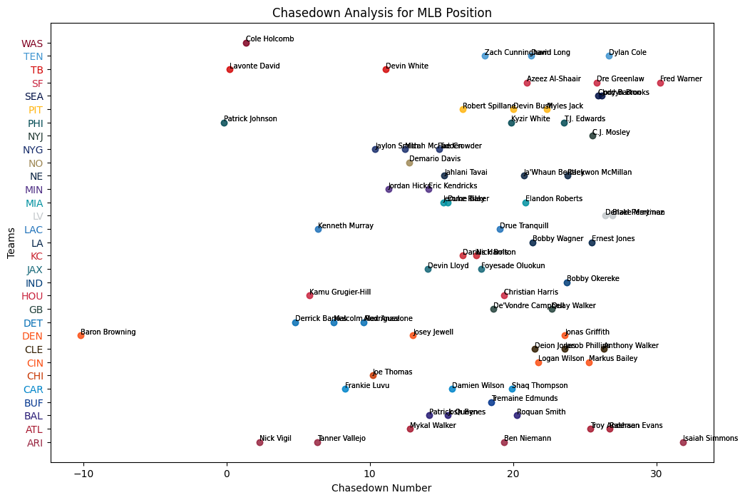
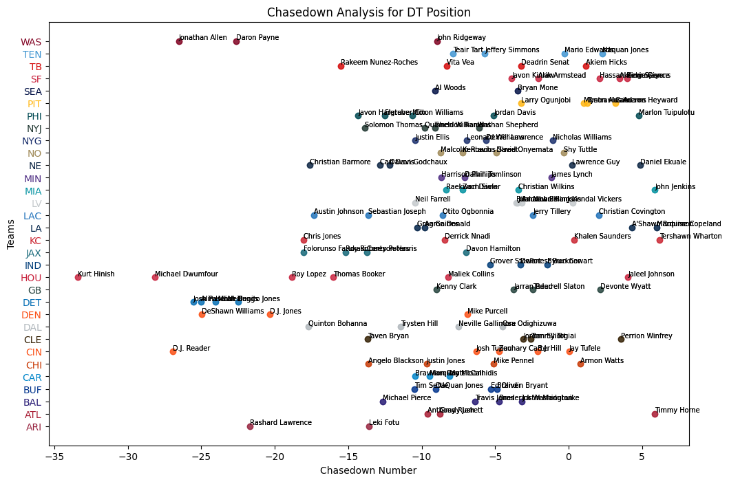
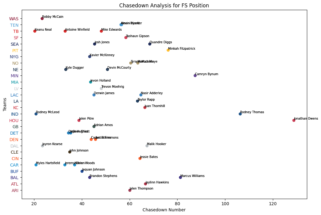
As you can see, SPEED is a stat that is highly correlated with position, making it useful in comparing players of the same position across teams. Players in the secondary have the highest SPEED values, followed by linebackers, and finally defensive lineman.
WATT
Congrats, you’ve mastered the art of pursuit. Now, the follow through - tackling. Once defenders are able to get in position to make the tackle, we need to assess how well they perform the tackle.
Intuitively, we thought a skewed normal distribution would best model tackle probabilities relative to defender, but this is not the case. After analyzing the position of the ball carrier relative to the tackler at the time of tackle for all tackles made, we conducted a Kolmogorov-Smirnov test and found that the T distribution best modeled this data, prompting us to model tackle probabilities of a defender using a bivariate T distribution as shown below.
K-S Test P Values for Skewed Normal Distribution and T Distribution for MLB:
- P-val x Skewnorm: 0.014822657499715244
-
P-val x T: 0.7394879983143571
- P-val y Skewnorm: 0.02577925347649812
- P-val y T: 0.970417444643622
Below, we inspect the middle linebackers’ distribution of tackles made relative to the player. The left plot shows where, relative to the player, the ball carrier was at the time of tackle. The right plot is the bivariate T distribution generated by fitting the data.
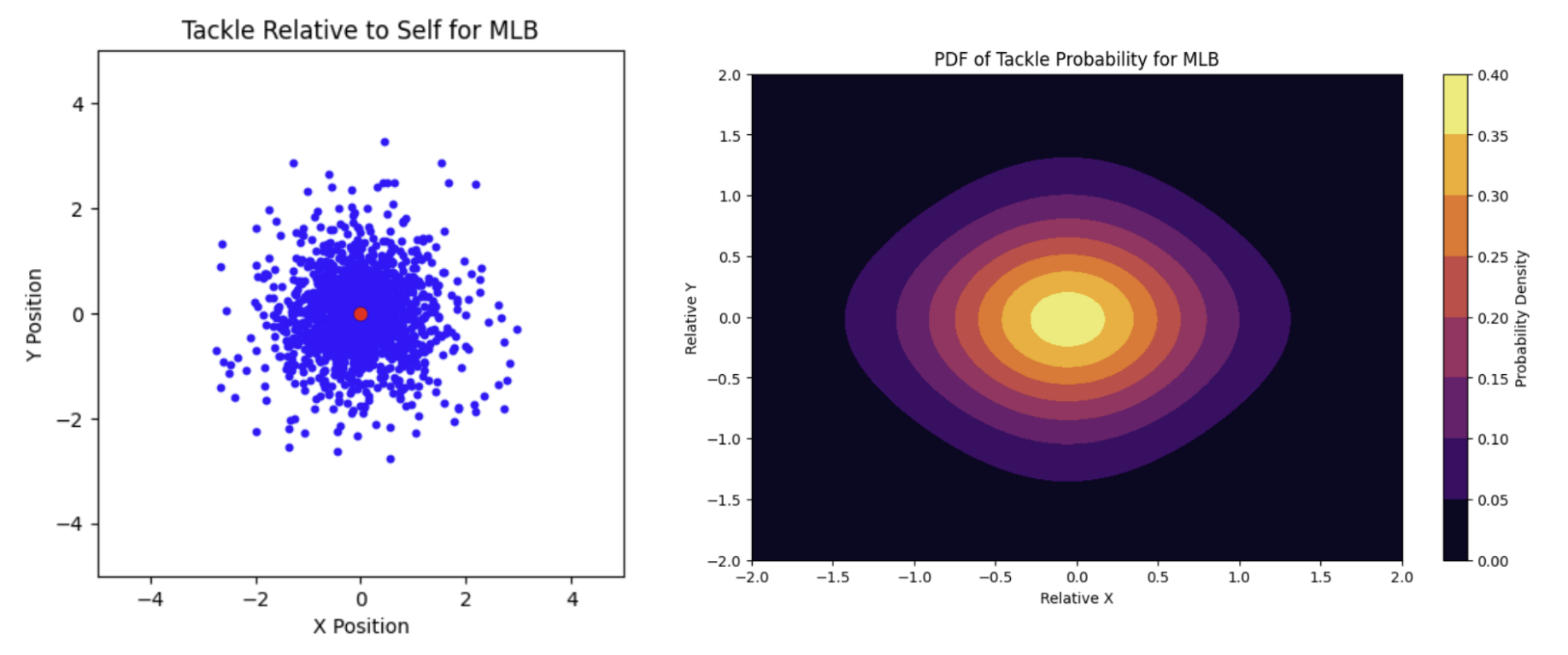
WATT generates a tackle probability distribution unique to each defensive position for each frame of a play. These distributions are dynamically updated to factor in offensive blocker position by scaling down proportionately to the defensive proportion of control on the area. The metric also incorporates offensive data which accounts for blockers being able to lower the probability of making a tackle. Throughout the course of the play, if the area of the distribution that overlaps with the ball carrier is greater than 50%, that defender has a chance to make a tackle, putting them in consideration as a potential tackler. Then based on if they made the tackle, missed the tackle, or didn’t do either, they are then scored, taking into account their average probability of making the tackle.
In this play, Ezekiel Elliott of the Cowboys makes a run against the Lions for a 12 yard gain. On the side, the animation shows the probability density function of each defender within proximity of Zeke. As the run goes on, we are able to see certain defenders’ PDF become more or less translucent, based on how much ground they gain or lose on Zeke, as well as how many offensive blockers are in front of them. By the end of the play, all defenders’ PDFs have been depleted, since none of them were able to tackle Zeke, thus being a very low scoring WATT play for the Cowboys defense.
VORTEX
Finally, to cap things off, we combine SPEED and WATT into our VORTEX plot. The plot is two-dimensional, with the x-axis being SPEED and the y-axis being WATT. This two-axis system allows for a more comprehensive assessment of a player’s overall defensive performance. Defenders who are both quick in pursuit (high SPEED) and effective at completing tackles (high WATT) will score well in both dimensions, identifying them as top defensive performers.
We will use cornerbacks, outside linebackers, and defensive tackles as examples, and show their VORTEX plots below.
As we can see in the VORTEX plot, different positions tend to cluster in different regions of the plot, reflecting the unique demands and responsibilities of each position. For instance, cornerbacks tend to have high SPEED but varying WATT scores, indicating that while they are often quick to pursue, their success in tackling can vary. Outside linebackers, on the other hand, tend to have a balance of both SPEED and WATT, reflecting their dual role in pass coverage and run defense. Defensive tackles usually have lower SPEED scores, but their WATT scores can vary widely, reflecting their primary role in stopping runs at the line of scrimmage.
Conclusion
In conclusion, the analysis and metrics presented offer a comprehensive framework for evaluating defensive performance in football. By focusing on both the pursuit (SPEED) and execution (WATT) of tackles, we can better understand and appreciate the contributions of defensive players. The VORTEX plot, in particular, provides a holistic view of player performance, allowing coaches, analysts, and fans to identify top performers and areas for improvement. This approach not only enhances our understanding of individual player performance but also offers valuable insights into team dynamics and defensive strategies. As we continue to refine and expand these metrics, we look forward to providing even deeper insights into the art and science of tackling in football.